Speed of model

Runtime is an important aspect of actuarial cash flow models. With the tight reporting deadlines, actuaries are keen to have results as fast as possible. In this post, we will discuss how to measure and improve the runtime of actuarial cash flow models.

List of content:

1. How to improve speed of model?
• Multiprocessing
• Indexing assumptions
• CSV reader
• Maximal calculation period
• Fit formulas
2. How to measure runtime?

How to improve speed of model?

Firstly, we will discuss how to improve the speed of the actuarial cash flow models. In particular, we will discuss the following aspects:

• multiprocessing,
• indexing assumptions,
• maximal calculation period,
• fit formulas.

Multiprocessing

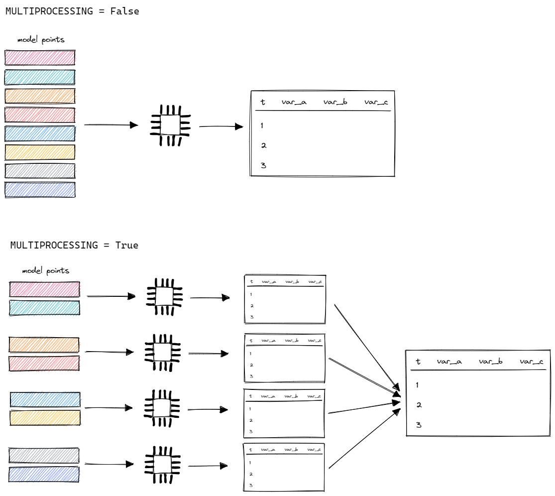
The model is evaluated for each model point one after another. It's also possible to calculate multiple model points at the same time and then to combine results. Modern computers have multiple cores that allow to perform calculations in parallel.

To turn on parallel calculations, set the MULTIPROCESSING setting to True.

# settings.py
settings = {
    # ...
    "MULTIPROCESSING": True,
    # ...
}

The model will split all model points into more or less equal parts, calculate them in parallel on multiple cores and then merge together into a single output. Thanks to that, the runtime will be decreased. The more cores, the faster calculation.

It is recommended to use MULTIPROCESSING when the model is stable. If you are developing the model, it's better to use single processing. The log messages might be vague, while multiprocessing.

Indexing assumptions

Reading data from external files impacts the runtime materially. To speed up reading data from assumptions files, we can use indexing.

Let's take a mortality table as an example. The first column is AGE and then there are two columns (MALE and FEMALE) with actual mortality rates.

# mortality.csv
AGE,MALE,FEMALE
0,0.00389,0.00315
1,0.00028,0.00019
2,0.00019,0.00014
3,0.00015,0.00011
4,0.00012,0.00009
..., ... ,...
96,0.28581,0.25969
97,0.30122,0.27829
98,0.31662,0.29696
99,0.33192,0.31554
100,0.34704,0.33387

In this table, we can set the AGE column as an index because we always read a mortality rate for the given age.

Let's do that:

# input.py
assumption = {
  "mortality": pd.read_csv("./input/mortality.csv", index_col="AGE")
}

Once we've set the index column, we can read data using the loc method:

# model.py
@variable()
def mortality_rate(t):
    sex = policy.get("SEX")
    if age(t) == age(t-1):
        return mortality_rate(t-1)
    elif age(t) <= 100:
        yearly_rate = assumption["mortality"].loc[age(t)][sex]
        monthly_rate = (1 - (1 - yearly_rate)**(1/12))
        return monthly_rate
    else:
        return 1

Let's take a closer look:

assumption["mortality"].loc[age(t)][sex]

We use loc to locate the given age in the index column and then choose the column indicated by sex (MALE/FEMALE).

Having an index in place improves the speed of reading data.

CSV reader

If you are reading data from a csv file, the CSVReader class can significantly speed up your data processing tasks.

The CSVReaderclass has some requirements:

• the row labels must be in the leftmost columns,
• row label(s) and column label must be provided as string,
• the return value is always a string so the developer should cast it to the appriopriate type.

In various scenarios, like actuarial practices, data tables often have row labels on the left side. Actuaries typically need to extract individual values from such tables. The CSVReader class is designed to leverage these characteristics and rapidly retrieve single values from the data.

The example usage of CSVReader:

# data.csv
X,A,B,C
1,1.1,2.2,3.3
2,4.4,5.5,6.6
3,7.7,8.8,9.9

from cashflower import CSVReader

reader = CSVReader("data.csv")
value = float(reader.get_value("2", "C"))  # Retrieves value 6.6

If the row label uses multiple columns, set the number of columns when initializing the class and provide a tuple while retrieving a value.

# data.csv
X,Y,1,2,3
1,1,4,5,7
1,2,9,2,4
2,1,3,5,2
2,2,3,9,6

from cashflower import CSVReader

reader = CSVReader("data.csv", num_row_label_cols=2)
value = int(reader.get_value(("2", "1"), "2"))  # Retrieves value 5

Maximal calculation period

By default, the maximal calculation is set to 720 (60 years). If such a long calculation horizon is not needed, then decrease it. You will get rid of unnecessary calculations that do not impact the result.

# settings.py
settings = {
    # ...
    "T_MAX_CALCULATION": 480,
    # ...
}

Fit formulas

While defining model variables, we should avoid unnecessary calculations. For example, we know that reading assumptions from tables takes time.

We could consider a different approach to the following formula.

@variable()
def mortality_rate(t):
    sex = main.get("SEX")
    if age(t) <= 100:
        yearly_rate = float(assumption["mortality"].loc[age(t)][sex])
        monthly_rate = (1 - (1 - yearly_rate)**(1/12))
        return monthly_rate
    else:
        return 1

We know that the age changes only every 12 months. There is no need to read data from the assumption table for the remaining 11 months.

We can add an if-statement that checks whether the age has changed:

if age(t) == age(t-1):
    return mortality_rate(t-1)

Thanks to that we save some computational time. Let's see the full formula.

@variable()
def mortality_rate(t):
    sex = main.get("SEX")
    if t > 0 and age(t) == age(t-1):
        return mortality_rate(t-1)
    elif age(t) <= 100:
        yearly_rate = float(assumption["mortality"].loc[age(t)][sex])
        monthly_rate = (1 - (1 - yearly_rate)**(1/12))
        return monthly_rate
    else:
        return 1

How to measure runtime?

The cashflower package produces a diagnostic file by default.

# settings.py
settings = {
    # ...
    "SAVE_DIAGNOSTIC": True,
    # ...
}

The model creates the <timestamp>_diagnostic.csv file in the output folder.

  .
  └── output/
      └── <timestamp>_diagnostic.csv

The diagnostic file contains different diagnostic information. One of these information is the runtime per variable.

# diagnostic
variable              runtime
survival_rate         10.84
expected_benefit      16.44
net_single_premium    12.99

We can analyze this file and check which variables take most of the runtime.