

With actuarial models, we try to predict the future by projecting cash flows over time. These models place results on a timeline with specific future dates, helping actuaries assess financial outcomes. Understanding how time is structured in cash flow models is important, as it affects calculations, assumptions, and financial projections.
The timeline typically starts at a valuation date and progresses in regular intervals, often monthly. Assumptions like interest rates and mortality rates are linked to specific time points or periods. In this post, we will explore how time is represented in actuarial cash flow models and discuss key time-related concepts.
Time in actuarial cash flow models
Timeline
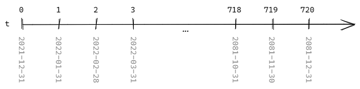
Let's start with the beginning. Timeline starts at zero (\( t=0 \)) which reflects the valuation period. If the reporting period is the end of year 2021, then \( t=0 \) is 2021-12-31.
We assume that \( t \) reflects certain point in time (as opposed to a period). The projections in cash flow models are usually monthly, so \( t=1 \) is 2022-01-31; \( t=2 \) is 2022-02-28; \( t=3 \) is 2022-03-31; etc.
The projection lasts for many years, for example, 60 or 100 years. The maximal projection is usually 120 years because it is assumed that the mortality rate at the age of 120 is 100% ( \( q_{120}=1 \) ).
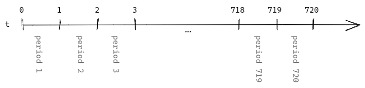
Periods
So far everything seems clear. A confusing aspect is that some assumptions concern periods rather than points in time.
Let's take interest rates as an example. Actuaries use interest rates to calculate the change in the value of money in time.
Let's say that we have €100 at \( t=2 \) (2022-02-28). The interest rate in March is 0.2%, so we have €100.20 at \( t=3 \) (2022-03-31). The interest rate is applied to a period from \( t=2 \) to \( t=3 \). So, should this assumption be linked to \( t=2 \) or \( t=3 \)?
It's likely that you will see the assumptions in the following way:
| time | interest rate |
|---|---|
| ... | ... |
| 3 | 0.002 |
| ... | ... |
We have linked the interest rate to the \( t=3 \), which is the end of the period. We may also think about this as a rate for the 3rd period.
Cash flows
You may have noticed that we assume that \( t \) is always the end of the month. Usually, we don't actually know the exact day in a month when the given cash flow occurs.
For example, a policyholder may pay premiums on different days of the month. If the terms of the policy say that the premium should be paid before the 10th day of the month, we can model it at the 10th. Policyholders may pay earlier, in that case, the present value will be higher.
Yet, premiums may occur during the whole month more or less uniformly. Then it makes sense to model them in the middle of the month. But how to model cash flow in the middle of the month if \( t \) only takes integer values? We can assign the nominal cash flow to the given \( t \) and reflect the fact that it happens in the middle of the month while discounting.
Let's go over an example. We have premiums occurring in January, February and March and we assign them to \( t=1, 2, 3 \) respectively.
| t | premium |
|---|---|
| 0 | 0 |
| 1 | 100 |
| 2 | 98 |
| 3 | 96 |
Since we know that premium payments occur uniformly during the month, it's sensible to model the cash flow in the middle of the month. We should then discount them accordingly.
If interest rate amounts to \( 0.002 \) (0.2%) for each of the months then monthly discount factor is \( v=1/(1+0.002) \). The first premium is discounted with \( v^{ \frac{1}{2} } \) , the second with \( v^{ \frac{3}{2} } \) and the third with \( v^{ \frac{5}{2} } \).
| t | premium | discount_factor | pv_premium |
|---|---|---|---|
| 0 | 0 | 1 | 0 |
| 1 | 100 | \( v^{ \frac{1}{2} } \) | 99.90 |
| 2 | 98 | \( v^{ \frac{3}{2} } \) | 97.71 |
| 3 | 96 | \( v^{ \frac{5}{2} } \) | 95.52 |
The present value of premiums amounts to € 293.13.
If the cash flow occurs at the end of the month then this approach is unnecessary. For example, some expenses are always due at the end of the month after the service has been provided. Then we should discount them normally.
| t | expense | discount_factor | pv_expense |
|---|---|---|---|
| 0 | 0 | 1 | 0 |
| 1 | 40 | \( v \) | 39.92 |
| 2 | 40 | \( v^{2} \) | 39.84 |
| 3 | 40 | \( v^{3} \) | 39.76 |
To sum up, the timeline is used in projection of future cash flows in actuarial models. Time is modelled with the \( t \) variable that reflects the time. The variable \( t \) takes integer values and they reflect the end of each month starting with the valuation period as the beginning. Some assumptions concern whole periods so the actuaries should be cautious to apply them correctly. Cash flows may happen over the whole period so it might make sense to model them in the middle of the month. We then need to discount them appropriately.
Time-related formulas
The time variable (t) is a system variable in actuarial cash flow models. The t variable represents monthly periods starting from zero.
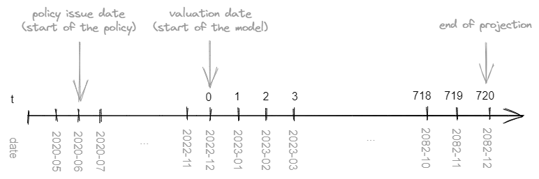
The model is run for the valuation date chosen by the actuary. The valuation date reflects the start of the model (t=0). The information on the valuation date can be stored in the runplan.
Below you can find model formulas for time-related variables that might be helpful in the model's development.
We will use the cashflower package in Python.
Calendar year and month
Knowing the valuation date, we can calculate actual calendar years and months. The valuation year and month can be read from the runplan. An example of input can be found in the later section. Here we have called these columns valuation_month and valuation_year.
# model.py
@variable()
def cal_month(t):
    if t == 0:
        return runplan.get("valuation_month")
    if cal_month(t-1) == 12:
        return 1
    else:
        return cal_month(t-1) + 1


@variable()
def cal_year(t):
    if t == 0:
        return runplan.get("valuation_year")
    if cal_month(t-1) == 12:
        return cal_year(t-1) + 1
    else:
        return cal_year(t-1)
Elapsed months
Each policy starts at a different moment. The policy's issue date might be part of the model points. Here the columns in model point set are called issue_year and issue_month. You can see an example of the model point set in the later section. Elapsed months reflect how many months have passed between the policy's issue and the valuation date.
# model.py
@variable()
def elapsed_months():
    issue_year = policy.get("issue_year")
    issue_month = policy.get("issue_month")
    valuation_year = runplan.get("valuation_year")
    valuation_month = runplan.get("valuation_month")
    return (valuation_year - issue_year) * 12 + (valuation_month - issue_month)
Policy year and month
Policy year and month reflect the duration of the given policy.
# model.py
import math

@variable()
def pol_month(t):
    if t == 0:
        mnth = elapsed_months() % 12
        mnth = 12 if mnth == 0 else mnth
        return mnth
    if pol_month(t-1) == 12:
        return 1
    return pol_month(t-1) + 1


@variable()
def pol_year(t):
    if t == 0:
        return math.floor(elapsed_months() / 12)
    if pol_month(t) == 1:
        return pol_year(t-1) + 1
    return pol_year(t-1)
Example
Input
Model uses runplan to store the information on the valuation date which is December 2022.
The policyholder has a policy that was issued in June 2020.
# input.py
import pandas as pd

from cashflower import Runplan, ModelPointSet

runplan = Runplan(data=pd.DataFrame({
    "version": [1],
    "valuation_year": [2022],
    "valuation_month": [12]
}))

policy = ModelPointSet(data=pd.DataFrame({
    "issue_year": [2020],
    "issue_month": [6],
}))
Results
The result for the first 13 months.
# output
  t  cal_month  cal_year  elapsed_months  pol_month  pol_year
  0         12      2022              30          6         2
  1          1      2023              30          7         2
  2          2      2023              30          8         2
  3          3      2023              30          9         2
  4          4      2023              30         10         2
  5          5      2023              30         11         2
  6          6      2023              30         12         2
  7          7      2023              30          1         3
  8          8      2023              30          2         3
  9          9      2023              30          3         3
 10         10      2023              30          4         3
 11         11      2023              30          5         3
 12         12      2023              30          6         3
 13          1      2024              30          7         3
Few things to note:
- cal_month, cal_year - starts with the valuation date,
- elapsed_months - the number of months between issue of the policy (2020-06) and the valuation date (2022-12),
- pol_month, pol_year - the policy was already 2 years and 6 months old at the valuation date.
Thank you so much for reading this tutorial! I hope you found it helpful and learned something new. If you have any questions or would like to share your thoughts, please leave a comment below or on github. Your feedback is valuable to us. Happy learning!