

Interest rates play a vital role in actuarial cash flow models by helping us figure out the value of money over time. In this blog post, we'll show you how to use interest rates in a Python cash flow model with a practical example.
Forward and spot rates
Interest rates curve
Often, when we first learn about the time value of cash flows, we're introduced to a single interest rate, like \( i=0.04 \) yearly. We say that \( 100 \) euros is worth \( 100 \cdot 1,04 = 104 \) euros in a year, \( 104 \cdot 1,04 = 108,16 \) in two years and so on.
However, in actuarial practice, we use interest rate curve rather than a single interest rate. Using interest rate curve means that we expect a different interest rate in each period.
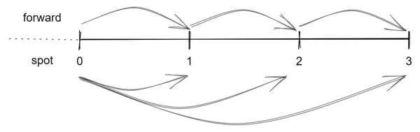
Interest rates can be represented in two primary ways: as forward rates and as spot rates. Forward rates denote the anticipated change in value between two future moments, while spot rates illustrate the expected change in value for a specific maturity.
Calculation example
Let's take a practical example. Here are the rates for the next three periods:
| period | forward | spot |
|---|---|---|
| \( 1 \) | \( 0.020000 \) | \( 0.020000 \) |
| \( 2 \) | \( 0.025000 \) | \( 0.022497 \) |
| \( 3 \) | \( 0.030000 \) | \( 0.024992 \) |
For this example, let's start with 100 euros.
First period
The value of that 100 euros after the first period is calculated in the same way using forward and spot rates.
Forward: \( 100 \cdot (1 + 0.02) = 102 \)Spot: \( 100 \cdot (1 + 0.02) = 102 \)
After the first period, we will have 102 euros.
Second period
We reinvest all the money, and after the second period, we have:
Forward: \( 100 \cdot (1 + 0.02) \cdot (1 + 0.025) = 104.55 \)Spot: \( 100 \cdot (1 + 0,022497)^2 = 104.55 \)
We now have 4.55 euros more than we started with.
Third period
Once again, we reinvest, and after the third period, we receive:
Forward: \( 100 \cdot (1 + 0.02) \cdot (1 + 0.025) \cdot (1 + 0.03) = 107.69 \)Spot: \( 100 \cdot (1 + 0.024992)^3 = 107.69 \)
At the end, we have 107.69 euros.
To calculate the time value of money using forward rates, we use all rates from the curve up to the given period. To calculate the time value of money with spot rates, we use only the rate for the given period.
Mathematical formula
We can use the following formula to calculate the future value ( \( FV \) ) of 1 euro after \( n \) periods using forward and spot rates:
Forward: \( FV_{n} = (1+f_{1}) \cdot (1+f_{2}) \cdot … \cdot (1+f_{n}) \)
Spot: \( FV_{n} = (1 + s_{n})^n \)
The formula for the forward rate in the period \( n \):
\( f_{n} = \frac{ (1+s_{n})^t }{ (1+f_{1}) \cdot (1+f_{2}) \cdot ... \cdot (1 + f_{n-1}) - 1} = \frac{ (1+s_{n})^t }{ (1+s_{n-1})^{t-1} - 1 }\)
If the rate are annual, then use the following formula to get monthly rates:
\( (1+f_{t})^{1/12}-1 \)
Modelling
Let's explore how to use interest rates curve in practice. For this, we'll leverage the cashflower package in Python.
Preparation
If you haven't already, please install the cashflower package using your terminal:
pip install cashflowerNext, let's create a dedicated model called interest_rates using Python:
from cashflower import create_model

create_model("interest_rates")
The create_model() function sets up the necessary file structure for our model:
interest_rates/
  input.py
  model.py
  run.py
  settings.py
Input
We will use the risk-free interest rates published by EIOPA. You can find the relevant file in the "Monthly Technical Information" section. For this tutorial, we have already prepared the data in the form of a csv file:
# input.py
import pandas as pd

assumption = {
    "interest_rates": pd.read_csv("./input/interest_rates.csv", index_col="T")
}
Let's take a look at the data:
print(assumption["interest_rates"]) VALUE
T
1 0.00736
2 0.01266
3 0.01449
4 0.01610
5 0.01687
.. ...
146 0.03191
147 0.03192
148 0.03194
149 0.03196
150 0.03198
Two important points to note:
- The data spans the next 150 years, which is sufficiently long since cash flow models typically cover periods of up to 120 years.
- These rates are annual, but our cash flow model operates with monthly periods, so we'll need to convert annual rates into monthly ones.
Model
Now, let's set up the core components of our financial model.
Projection year
We need to define a projection year to read the corresponding interest rate.
# model.py
@variable()
def projection_year(t):
    if t == 0:
        return 0
    elif t % 12 == 1:
        return projection_year(t-1) + 1
    else:
        return projection_year(t-1)
The projection year starts at zero and increments by one at the beginning of each year.
Yearly spot rate
We can now read the yearly spot rates from our assumption table using the projection year:
# model.py
@variable()
def yearly_spot_rate(t):
    if t == 0:
        return 0
    else:
        return assumption["interest_rates"].loc[projection_year(t)]["VALUE"]
For example, the interest rate for the first year is 0.736%, indicating that €100 will be worth €100.74 after a year.
Yearly forward rate
The yearly forward rate is calculated based on the yearly spot rates.
# model.py
@variable()
def yearly_forward_rate(t):
    if t == 0:
        return 0
    elif t == 1:
        return yearly_spot_rate(t)
    elif t % 12 != 1:
        return yearly_forward_rate(t-1)
    else:
        return ((1 + yearly_spot_rate(t))**projection_year(t)) / ((1 + yearly_spot_rate(t-1))**projection_year(t-1)) - 1
Monthly forward rate
Since our model operates on a monthly basis, we also need to calculate the monthly forward rate. This is done as follows:
# model.py
@variable()
def forward_rate(t):
    return (1+yearly_forward_rate(t))**(1/12)-1
Discount rate
To calculate the present value of future cash flows, we need discount rates. In our cash flow models, we use discount rates that apply for one period at a time:
# model.py
@variable()
def discount_rate(t):
    return 1/(1+forward_rate(t))
This formula calculates the discount rate for each period, allowing us to determine the present value of cash flows.
Cash flows
Now that we have our model structure in place, let's create and calculate the values for two payment streams, payment1 and payment2.
# model.py
@variable()
def payment1(t):
    if t == 0:
        return 100
    else:
        return 0

@variable()
def payment2(t):
    if t == 24:
        return 250
    else:
        return 0

@variable()
def future_value_payment1(t):
    if t == 0:
        return payment1(t)
    return payment1(t) + future_value_payment1(t-1) * (1+forward_rate(t))

@variable()
def present_value_payment2(t):
    if t == settings["T_MAX_CALCULATION"]:
        return payment2(t)
    return payment2(t) + present_value_payment2(t+1) * discount_rate(t+1)
These variables represent two payment streams. The first payment is a payment of €100 at the beginning of the projection, while the second payment is a payment of €250 after 2 years (24 months). We've also calculated future and present values based on the interest rates and discount rates.
Results
To view the results of our calculations, source the run.py script.
# output
 t  projection_year  yearly_spot_rate  yearly_forward_rate  forward_rate  discount_rate  payment1  payment2  future_value_payment1  present_value_payment2
 0              0.0           0.00000             0.000000      0.000000       1.000000     100.0       0.0             100.000000              243.788209
 1              1.0           0.00736             0.007360      0.000611       0.999389       0.0       0.0             100.061127              243.937231
 2              1.0           0.00736             0.007360      0.000611       0.999389       0.0       0.0             100.122292              244.086343
 3              1.0           0.00736             0.007360      0.000611       0.999389       0.0       0.0             100.183494              244.235547
 4              1.0           0.00736             0.007360      0.000611       0.999389       0.0       0.0             100.244734              244.384842
 5              1.0           0.00736             0.007360      0.000611       0.999389       0.0       0.0             100.306011              244.534228
 6              1.0           0.00736             0.007360      0.000611       0.999389       0.0       0.0             100.367325              244.683705
 7              1.0           0.00736             0.007360      0.000611       0.999389       0.0       0.0             100.428677              244.833274
 8              1.0           0.00736             0.007360      0.000611       0.999389       0.0       0.0             100.490067              244.982934
 9              1.0           0.00736             0.007360      0.000611       0.999389       0.0       0.0             100.551494              245.132686
10              1.0           0.00736             0.007360      0.000611       0.999389       0.0       0.0             100.612958              245.282529
11              1.0           0.00736             0.007360      0.000611       0.999389       0.0       0.0             100.674460              245.432464
12              1.0           0.00736             0.007360      0.000611       0.999389       0.0       0.0             100.736000              245.582490
13              2.0           0.01266             0.017988      0.001487       0.998515       0.0       0.0             100.885771              245.947616
14              2.0           0.01266             0.017988      0.001487       0.998515       0.0       0.0             101.035766              246.313284
15              2.0           0.01266             0.017988      0.001487       0.998515       0.0       0.0             101.185983              246.679496
16              2.0           0.01266             0.017988      0.001487       0.998515       0.0       0.0             101.336423              247.046252
17              2.0           0.01266             0.017988      0.001487       0.998515       0.0       0.0             101.487088              247.413553
18              2.0           0.01266             0.017988      0.001487       0.998515       0.0       0.0             101.637976              247.781401
19              2.0           0.01266             0.017988      0.001487       0.998515       0.0       0.0             101.789088              248.149795
20              2.0           0.01266             0.017988      0.001487       0.998515       0.0       0.0             101.940425              248.518738
21              2.0           0.01266             0.017988      0.001487       0.998515       0.0       0.0             102.091988              248.888228
22              2.0           0.01266             0.017988      0.001487       0.998515       0.0       0.0             102.243775              249.258268
23              2.0           0.01266             0.017988      0.001487       0.998515       0.0       0.0             102.395788              249.628859
24              2.0           0.01266             0.017988      0.001487       0.998515       0.0     250.0             102.548028              250.000000
25              3.0           0.01449             0.018160      0.001501       0.998501       0.0       0.0             102.701939                0.000000
Now it's finally time to take a look at the results.
Few things to note:
- projection year - it increases by 1 every 12 months,
- yearly spot rate - we read values from assumptions; these are yearly rates so there is the same value for the consecutive 12 months,
- yearly forward rate - it has the same value for the first year as yearly spot rate and changes afterwards,
- forward rate - it's a monthly rate, it has the same value for each projection year,
- discount rate - similar to forward rate, it's a monthly rate with the same value for each projection year,
- future_value_payment1 - value of the payment1 increases each month; the value for t=24 could be calculated also as 100 * (1+yearly_spot_rate(t=24))**2,
- present_value_payment2 - the payment hasn't happened yet, it will happen at t=24 but we can calculate what this money is worth for us now at t=0.
Thanks for reading this tutorial! I hope it was helpful. Feel free to leave a comment below or on github with any questions or thoughts. Your feedback matters. Happy learning!