Deterministic and stochastic models

Insurance companies rely on two main approaches for cash flow modelling: deterministic and stochastic. These models help estimate future liabilities of insurance products, guiding actuaries in predicting the future using historical data and expert judgment.

List of content:

1. Deterministic vs stochastic
2. Modelling example
• Problem
• Deterministic modelling
• Stochastic modelling

Deterministic vs stochastic

Imagine predicting the future: one way is to follow the most likely path, while the other is like exploring various possible paths, akin to the multiverse concept in Spiderman, where multiple worlds have slightly different versions of Peter Parker.

• Deterministic approach

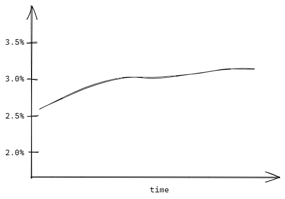
In the deterministic approach, we calculate the model on a single set of assumptions, like using one interest rates curve.

• Stochastic approach

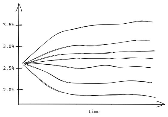
In the stochastic approach, we calculate the model on muliple sets of market assumptions, like multiple interest rates curves, and averages the results.

Practical use

Stochastic models often involve variations in market assumptions. They are commonly employed to assess the time value of guarantees (TVOG).

Consider a policy with a guaranteed return rate of 1% on a fund. If the interest rate surpasses 1%, the company faces no losses due to guarantees. However, if it falls below 1%, the guarantees might impact the company.

In a deterministic approach, the model might yield a TVOG result of zero. But in the stochastic approach, the company could face guarantee-related issues in certain scenarios.

Modelling example

We'll illustrate the stochastic approach using a simple example of discounting premiums, employing Python's cashflower package. If you're new to this package, refer the user guide.

Problem

Our goal is to calculate the present value of a set of premiums over a three-period projection, totaling four payments: one at the beginning of the projection and three after each consecutive period.

settings = {
  "T_MAX_CALCULATION": 3,
}

The initial premium amounts to 1000 and increases by 3% after each period.

main = ModelPointSet(data=pd.DataFrame({
    "id": [1],
    "initial_premium": [1_000],
}))

assumption = {
    "indexation": 0.03,
    # ...
}

The premium increases by the indexation rate in each subsequent period.

from input import main, assumption


@variable()
def premium(t):
    if t == 0:
        return main.get("initial_premium")
    else:
        return premium(t-1) * (1+assumption["indexation"])

Deterministic modelling

In deterministic modelling, we will use one path of discount rates.

assumption = {
    # ...
    "discount_rates": [1, 0.94, 0.96, 0.95]
}

We get the discount rates from the assumptions and calculate the present value.

@variable()
def discount_rate(t):
    return assumption["discount_rates"][t]


@variable()
def pv_premiums(t):
    if t == settings["T_MAX_CALCULATION"]:
        return premium(t)
    else:
        return premium(t) + pv_premiums(t+1) * discount_rate(t+1)

Stochastic modelling

In stochastic modelling, we don't have a single scenario for interest rates; instead, we anticipate multiple possible scenarios. In our example, we will consider two equally possible variations of interest rate:

• interest rates increase (discount rates decrease),
• interest rates decrease (discount rates increase).

assumption = {
    # ...
    "discount_rates1": [1, 0.92, 0.93, 0.91],
    "discount_rates2": [1, 0.97, 0.99, 0.98]
}

In this case, we calculate the model for both scenarios and average the results.

We will show two ways of how to calculate results for the stochastic approach in Python:

1. Manual - manual creation of separate variables for each of the scenarios,
2. Stochastic variables - by using stochastic variables.

Both ways generate the same results.

1. Manual

We create separate variables for each scenario and then derive a single estimate by averaging the results.

@variable()
def discount_rate1(t):
    return assumption["discount_rates1"][t]


@variable()
def discount_rate2(t):
    return assumption["discount_rates2"][t]


# Separate present value calculations for each scenario

@variable()
def pv_premiums1(t):
    if t == settings["T_MAX_CALCULATION"]:
        return premium(t)
    else:
        return premium(t) + pv_premiums1(t+1) * discount_rate1(t+1)


@variable()
def pv_premiums2(t):
    if t == settings["T_MAX_CALCULATION"]:
        return premium(t)
    else:
        return premium(t) + pv_premiums2(t+1) * discount_rate2(t+1)

# Average of results for a single estimate

@variable()
def pv_premiums_avg(t):
    return (pv_premiums1(t) + pv_premiums2(t)) / 2

2. Stochastic variables

For numerous possible paths, we can avoid creating separate variables by using cashflower's stochastic variables.

To use stochastic variables, firstly determine the number of stochastic scenarios in the settings.

settings = {
    "NUM_STOCHASTIC_SCENARIOS": 2,
}

Now, we define stochastic variables for discount rates and the present value of premiums, allowing for calculations for each scenario separately and averaging the results.

@variable()
def discount_rate(t, stoch):
    return assumption["discount_rates"+stoch][t]


@variable()
def pv_premiums(t, stoch):
    if t == settings["T_MAX_CALCULATION"]:
        return premium(t)
    else:
        return premium(t) + pv_premiums(t+1, stoch) * discount_rate(t+1, stoch)

The cashflower calculates discount rates and present value for each scenario independently before averaging the results.

Thank you for taking the time to read this post! I hope you found it interesting and informative. Feel free to share your thoughts by leaving a comment below. If you have any questions or want to engage further, head over to the discussions section of the repository. Your feedback and contributions are always appreciated!